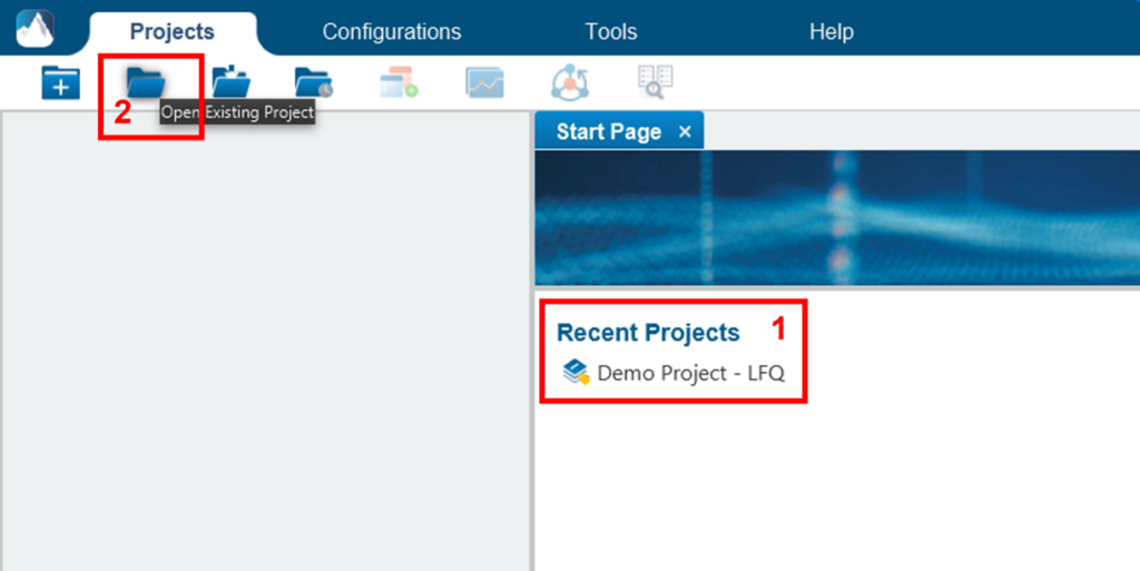
Instructions for the installation of PEAKS can be found in “Chapter 2, Installation and Activation” of the User Manual. After installation and running PEAKS, you can open the sample project by one of the following two ways (see screenshot below):

1. If this is a fresh installation, click the “Sample Project” in the “Recent Projects” list of the Start Page.
2. Click the open project button, and browse to the directory where PEAKS was installed, select “SampleProject” and click the open button in the file browser.

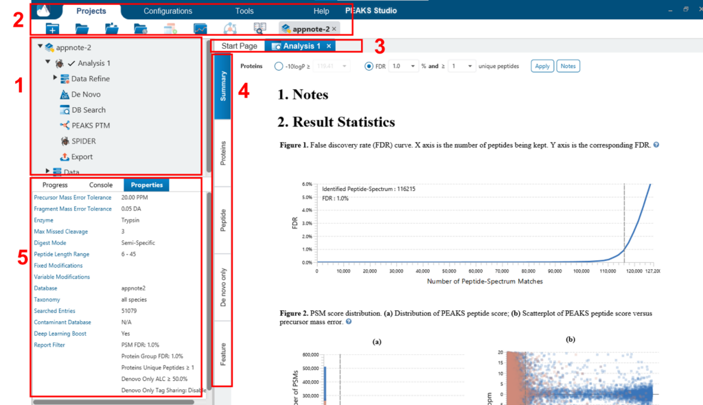
The main graphical user interface (GUI) of PEAKS is divided into the following areas (see screenshot below):

1. In Project View tree will display any opened projects that are complete or in progress and show the analysis under the project. Each analysis can collapse/expand. Selecting a node (project, sample, fraction, or result) in an opened project will highlight the analysis tool icons that are available to the selected node.
2. Double clicking the result node (third level, such as Data Refine, De Novo, DB search, etc.) to open the result. Opened result nodes are shown in tabs.  Right clicking on the analysis node provides the option to change the name of the Analysis. There is also an option to delete the analysis from the project..
3. Each opened result node provides several different “views” as different tabs. In particular, the “Summary View” shows the result statistics and is also the central tab in which to filter and export PEAKS results.
4. The information pane to show useful information such as node property and progresses of running tasks.
5. The menu and toolbar contain all of the analysis tool icons.

After double-clicking to open a result node (e.g., the PEAKS DB node in the sample project) the “Summary View” is shown by default and provides mainly three functions:

1. Specify score thresholds to filter the results
2. Examine the result statistics
3. Export results

The top region of the “Summary View” is a control pane in which the results are controlled (see screenshot below), and the bottom region is a statistics report page:

• Low scoring peptide identifications are filtered out by setting a desired peptide-spectrum match -10lgP threshold or a desired FDR (false-discovery rate), which can be specified by clicking the FDR button.
• Low scoring protein identifications are filtered out by setting a desired protein -10lgP score and a desired unique peptide count.
• The de novo only peptides are those with confident de novo sequence tags that remain unidentified by the database search algorithms. To report a de novo only peptide, the ALC (average local confidence) scores must be equal to or better than the specified threshold. Meanwhile, the score of the spectrum’s best database search result should be no greater than the specified -10lgP threshold.
• By default, the -10logP threshold used for de novo only is locked to be the same as the -10lgP threshold used for filtering peptides. To specify a different value, simply click the lock icon to unlock the filter.

After the filtration criteria are changed, the Apply Filters will change to red. Click it to apply the new criteria.

The top control pane has two additional buttons: Export and Notes. Clicking Export displays several options and file formats in which a user can export analysis results. Clicking Notes allows the user to add a text note about the project which will be displayed at the top of the “Summary” view page and in the HTML export.

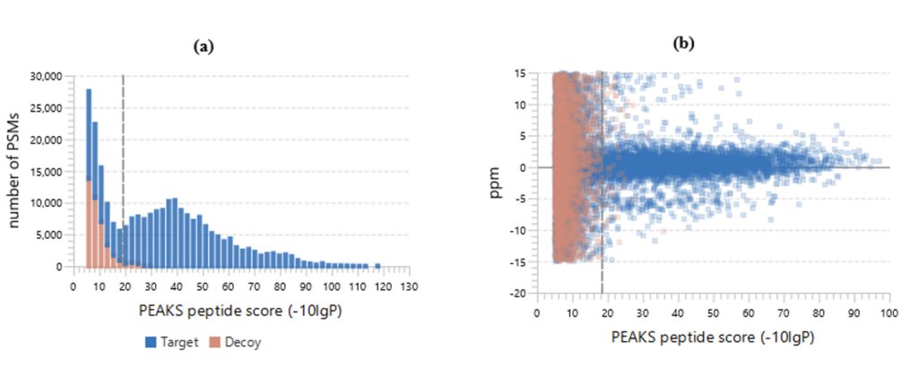
After applying the filters, the statistics report page at the bottom of the “Summary” view will be updated accordingly. Only two statistical charts are explained here (see screenshot below).

Figure 2(a) shows the PSM score distribution in a stacked histogram. If both the search result and the peptide -10lgP score threshold are of high confidence, very few decoy matches (brown) in the high score region should be observed. Additionally, if the FDR estimation method (decoy fusion) worked properly, then a similar or greater number of decoy (brown) matches should be observed in the low score region relative to the target (blue) matches.

Figure 2 (b) plots the precursor mass error v.s. -10lgP peptide score for all PSMs. This figure is the most useful for the high resolution instruments. Generally, the high-scoring points should be centered around the mass error of 0. Notice that the data points start to scatter to larger mass errors when they are below a certain score threshold.

In addition to the “Summary View”, PEAKS organises its results into five sections: “Feature”, “Protein”, “Peptide”, “De Novo Only”, and “LC/MS”.

• The “Feature View” contains a list of all detectable features that passed the filters. Each feature will list all the MS/MS scans associated with it.
• The “Protein View” contains a list of proteins that passed the filters. The proteins identified with the same set (or a subset of) peptides are grouped together.
• The “Peptide View” shows all the peptide identifications passing the filters. The multiple spectra that identified the same peptide sequence are grouped together.
• The “De Novo Only View” shows all of the peptides identified exclusively by de novo sequencing.
• The “LC/MS View” displays the LC-MS data as a heat map with highlighted MS/MS scans and detected features.

Here, the focus will be on the protein coverage view only. Click the “Protein View” tab and select one protein. The corresponding protein coverage map will be displayed at the bottom of the “Protein View”. The protein coverage view maps all peptide identifications of the selected protein onto the protein sequence. It enables the effortless examination of every PTM and mutation on each amino acid. Some of the most commonly used operations on the protein coverage view are listed in the following (see screenshot below):

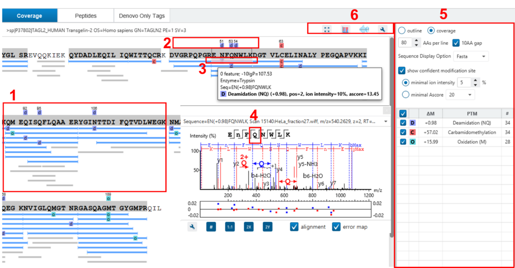
1. Each blue bar indicates an identified peptide sequence. A grey bar indicates a de novo only tag match.
2. PTMs and mutations are highlighted with coloured icons and white letter boxes. Highly confident PTMs and mutations are displayed on top of the protein sequence.
3. Click a peptide to show the spectrum annotation.
4. Hold the mouse over an amino acid to show the supporting fragment ion peaks.
5. Options to control the coverage view display.
   • The “coverage/outline” choice enables the display or the removal of the peptide bars.
   • The “sequence display option” highlights the coverage map based on either a fasta display or an enzyme display from one of the enzyme options selected during the project setup.
   • The “de novo tags sharing” specifies the minimum number of consecutive amino acid matches between a de novo only sequence and the protein before it can be displayed as a grey bar.
   • The “de novo peptides fully matched” check box allows a de novo peptide to be displayed if the sequence, regardless of its length, is fully matched to a sequence in the protein.
   • The “minimum ion intensity” specifies the minimum fragment ion relative intensity in one of the MS/MS spectra before a PTM location is regarded as confident and displayed on top of the protein sequence.
   • The check boxes in the PTM list allow users to view peptides with specific PTMs in the results. Click the colored boxes to change a colour. Double-click a PTM name to see the PTM detail.
6. The full screen button, the PTM profile button, the peptide mapping button, and the tool box button:

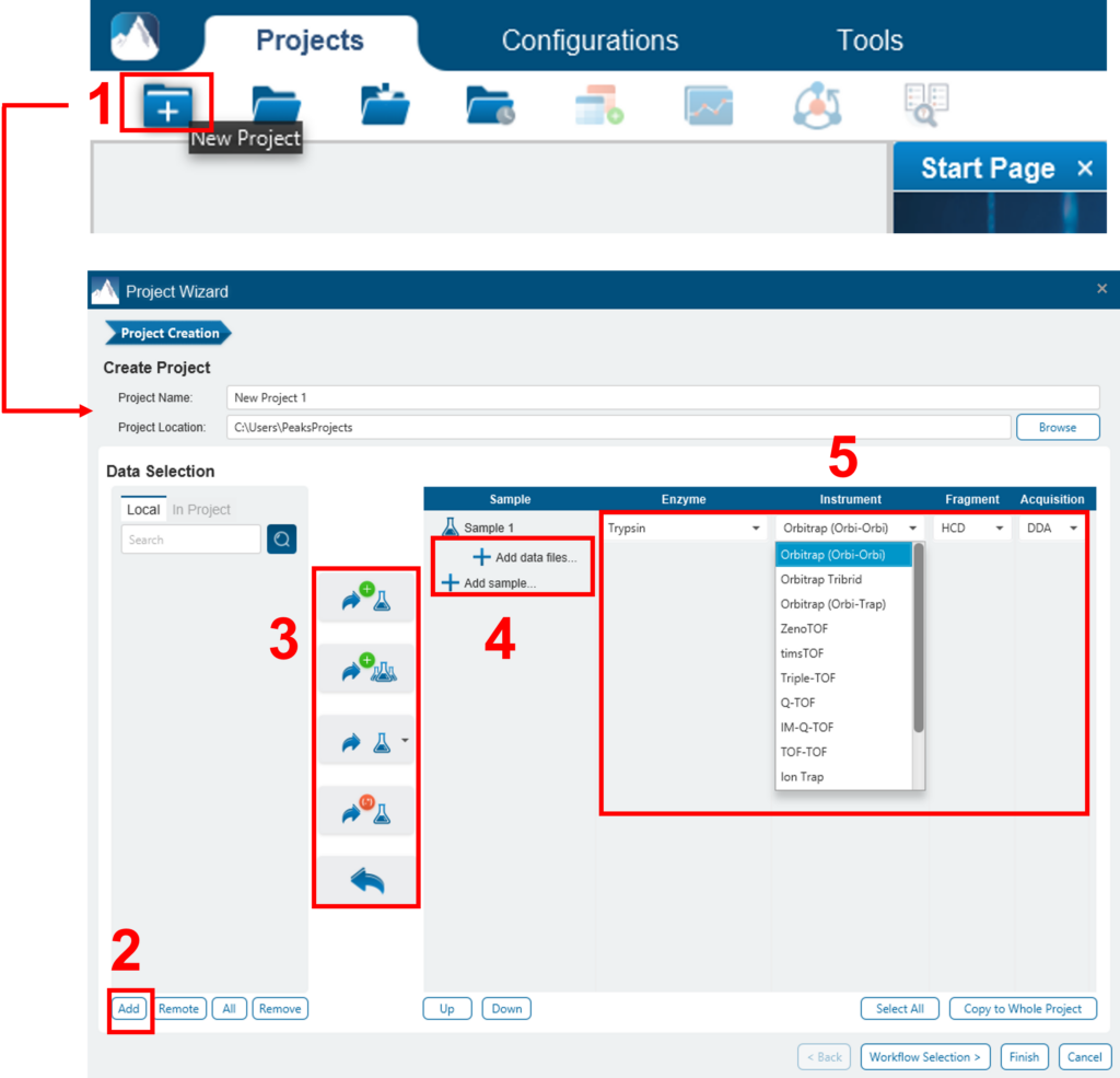
To create a new PEAKS project from raw data files, perform the following steps (see screenshot below):

1. Select New Project … from the file menu or click the New Project icon  on the tool bar. The “Project Wizard” will appear.
2. Use the Add Data button to add the desired files to be loaded, and then click Open. All of the selected data files will be listed on the left side.
3. Place the selected data from the list into samples: use  to place all files in a new sample; use  to put them in an existing sample; or put them in individual samples for each file using . If you want group files by delimiter or RegEx, you can click the button.
4. Click the  or the  buttons to add a sample to the project or data files to a sample, respectively.
5. For each sample, specify the sample details: “Instrument” type, “Fragmentation” method, “Enzyme” name, and Data “Acquisition”.
   • Note: Users can specify a different proteolytic enzyme per sample. Using multiple enzymes to analyse the same proteins can produce overlapping peptides, which will increase protein coverage.
   • Note: To apply the same sample details to the whole project, select the sample with the correct settings and click on the Copy to Whole Project button.
6. Click the Finish button to create the project

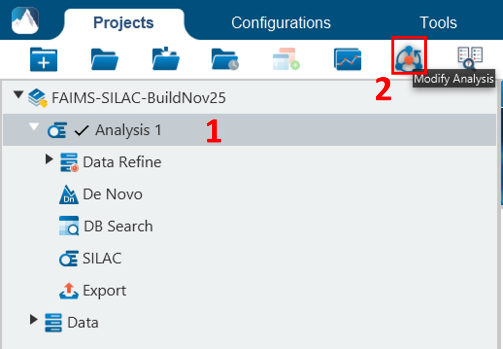
To conduct an analysis: 1) Select a project, a sample, or a result node in the Project View; 2) Click the desired analysis tool button. In the following example, the completed de novo result is selected from the Project View pane, and a PEAKS DB search will be employed using those results. The PEAKS DB is a workflow performing a database identification search.

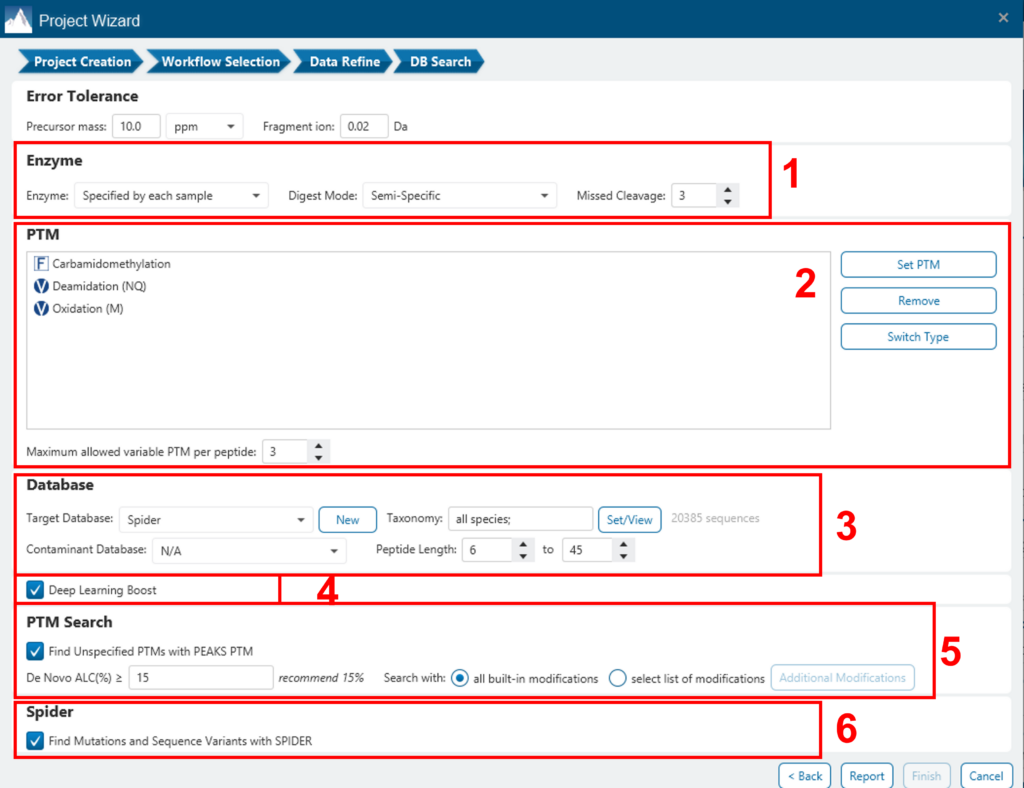
A window will appear to allow users to specify the desired search parameters for the analysis. Most search options for PEAKS DB are standard and straightforward. More details are provided in the following:

1. If the proteolysis enzyme was specified for each sample at the project creation step, users can choose to use the enzyme already specified in each sample. This makes it possible to use multiple enzymes in a single project and a single search.
2. Specify the fixed PTMs and a few common variable PTMs expected in the sample.
3. Select a protein sequence database, or copy and paste the protein sequences for the database search. Users can also select a contaminant database to be included in the database search (optional).
4. Conduct de novo sequencing using the same parameters or base the search on an existing de novo sequencing result node.
5. Estimate the false discovery rate (FDR) with the decoy fusion method.
   • Decoy fusion is an enhanced target-decoy method for result validation with FDR. Decoy fusion appends a decoy sequence to each protein as the “negative control” for the search. See BSI’s web tutorial for more details.
6. Enable PEAKS PTM and SPIDER algorithms after the PEAKS DB database search completes.
   • By default, PEAKS PTM will perform an additional PTM search, which considers all 313 naturally occurring modifications from Unimod. Users can instead specify a custom list of PTMs they wish to be used for the additional PEAKS PTM search by clicking the “Advanced Setting” button.
   • SPIDER performs a homology search based on de novo sequencing tags. If selected, SPIDER algorithm will be conducted on every confident de novo tag (ALC > 15%) whose spectrum is not identified by PEAKS DB with high confidence (-10lgP < 30). SPIDER will construct new peptide sequences by altering amino acids of database peptides. For each spectrum, the better sequence constructed by SPIDER or found by PEAKS DB will be used as the identified peptide. SPIDER is good for cross-species searches and for finding point mutations of the protein. SPIDER can either be invoked through this work flow or by clicking the SPIDER icon in the toolbar.